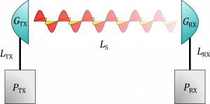
Link analysis – Andøya Space Education

Figure 1: A simplified overview of important link factors in a telemetry system. ‘TX’ and ‘RX’ refers to ‘transmitter’ and ‘receiver’, respectively. $P$ is the power exiting/entering the transmitter/receiver, $G$ is the gain of the antennas and $L_\text{S}$ is any losses ‘outside’ the transmitter and receiver, such as air damping, pointing loss or polarization mismatch. $L_\text{TX}, L_\text{RX}$ are the losses happening between the transmitter or receiver and its respective antenna. Illustration by Andøya Space Education.

The ultimate goal of telemetry is to transfer a perfect signal copy from A to B. Practically speaking, however, an acceptable level of information loss must be balanced against power usage, transmission speed and other limiting factors (e.g. available bandwidth and budget). This motivates a theoretical study of the connection quality between sender and receiver—i.e. ‘link analysis’—and the concept of a ‘link budget’—a systematic accounting of how signal power propagates throughout the system.

Connection quality can be evaluated by several metrics differing in refinement, generality and computational complexity. Ultimately, the goal is to determine how much power the transmitter needs and/or how sensitive the receiver apparatus needs to be in order to keep the error rate (or equivalently, the likelihood of a transmission error) sufficiently minimized. The error rate depends on the signal-to-noise ratio—the ratio between received signal power and noise power, often written S/N or SNR—which itself, aside from some complicating factors related to what is meant by a ‘signal’, depends on the received power $P_\text{RX}$ , which can be estimated by setting up a so-called link budget (of course, the signal-to-noise ratio also depends on the total noise power $N$ , but estimating noise is outside the scope of this article).

Using physical units (see below), a simplified link budget without noise takes the form

$\displaystyle P_\text{RX} = P_\text{TX} \cdot \frac{\displaystyle \prod G}{\displaystyle \prod L},$

where $P_\text{TX}$ is the transmitted power, $\prod G$ the product of all amplification factors and $\prod L$ the product of all loss factors.

When setting up a link budget, we are only interested in what happens after the signal exits the last electrical amplifier in the transmitter and before it enters the first electrical amplifier in the receiver. Hence, assuming that the transmitting antenna is passive, the total radiated power is at best (i.e. when assuming no loss in the antenna) given by

$\displaystyle P_\text{rad} = \frac{P_\text{TX}}{L_\text{TX}},$

where $L_\text{TX}$ is the line loss between the transmitter terminals and the antenna.

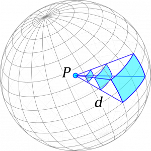Figure 2: The power $P$ of an isotropic antenna radiates outwards as a sphere. Hence, at a distance $d$ the received flux is $P/(4 \pi d^2)$ . Illustration by Andøya Space Education.

If we assume the transmitter antenna is isotropic—i.e. that it radiates equally in all directions (see figure 2)—and that the radiative medium can be treated as a vacuum, the received power becomes

$\displaystyle P_\text{RX} = \frac{P_\text{rad} \cdot A_\text{RX}}{4\pi d^2}\cdot \frac{1}{L_\text{RX}},$

where $A_\text{RX}$ is the effective area of the receiving antenna, $d$ is the distance between the two antennas and $L_\text{RX}$ is the line loss between the antenna and the receiver. If the receiving antenna is lossless and isotropic, it can be shown that its effective area is

$\displaystyle A_\text{iso} = \frac{\lambda^2}{4 \pi},$

where $\lambda$ is the wavelength of the received electromagnetic radiation.

Together, the three last equations gives an expression for the received power $P_\text{RX}$ under the assumption of lossless isotropic antennas in a vacuum. Accounting for anisotropy and antenna losses is done simply by multiplying by the antenna gains, as the gain of an antenna is defined by the power ratio between the actual, lossy anisotropic antenna and an ideal, lossless isotropic antenna. The effects of the environment and other mismatches between the antennas can be modeled as a product of loss factors $\prod L$ . Hence, we finally obtain the transmission equation

$\displaystyle P_\text{RX} = \frac{\displaystyle P_\text{TX} \, G_\text{TX}\, G_\text{RX}}{\displaystyle (4 \pi d / \lambda)^2 \, L_\text{RX} \, L_\text{TX} \, \prod L} = \frac{\displaystyle P_\text{TX} \, G_\text{TX}\, G_\text{RX}}{\displaystyle L_0 \, L_\text{RX} \, L_\text{TX} \, \prod L},$

where we introduced the so-called free-space path loss $L_0$ , which, for an electromagnetic wave with wavelength $\lambda$ , models the path loss between two lossless isotropic antennas separated by a distance $d$ in a vacuum:

$\displaystyle L_0 = \left(\frac{4\pi d}{\lambda}\right)^{\!2}=\left(\frac{4\pi d f}{c}\right)^{\!2} \! .$

It should be noted that the frequency dependence of the ‘free-space path loss’ does not reflect how ‘easily’ electromagnetic waves propagate in a vacuum—according to our best measurements, this is completely frequency independent—but rather how much electrical power an antenna can capture from a radiative field.

Other losses

Apart from the effects mentioned above, real-world telemetry systems are subject to several additional sources of signal attenuation and degradation (this list is not exhaustive!):

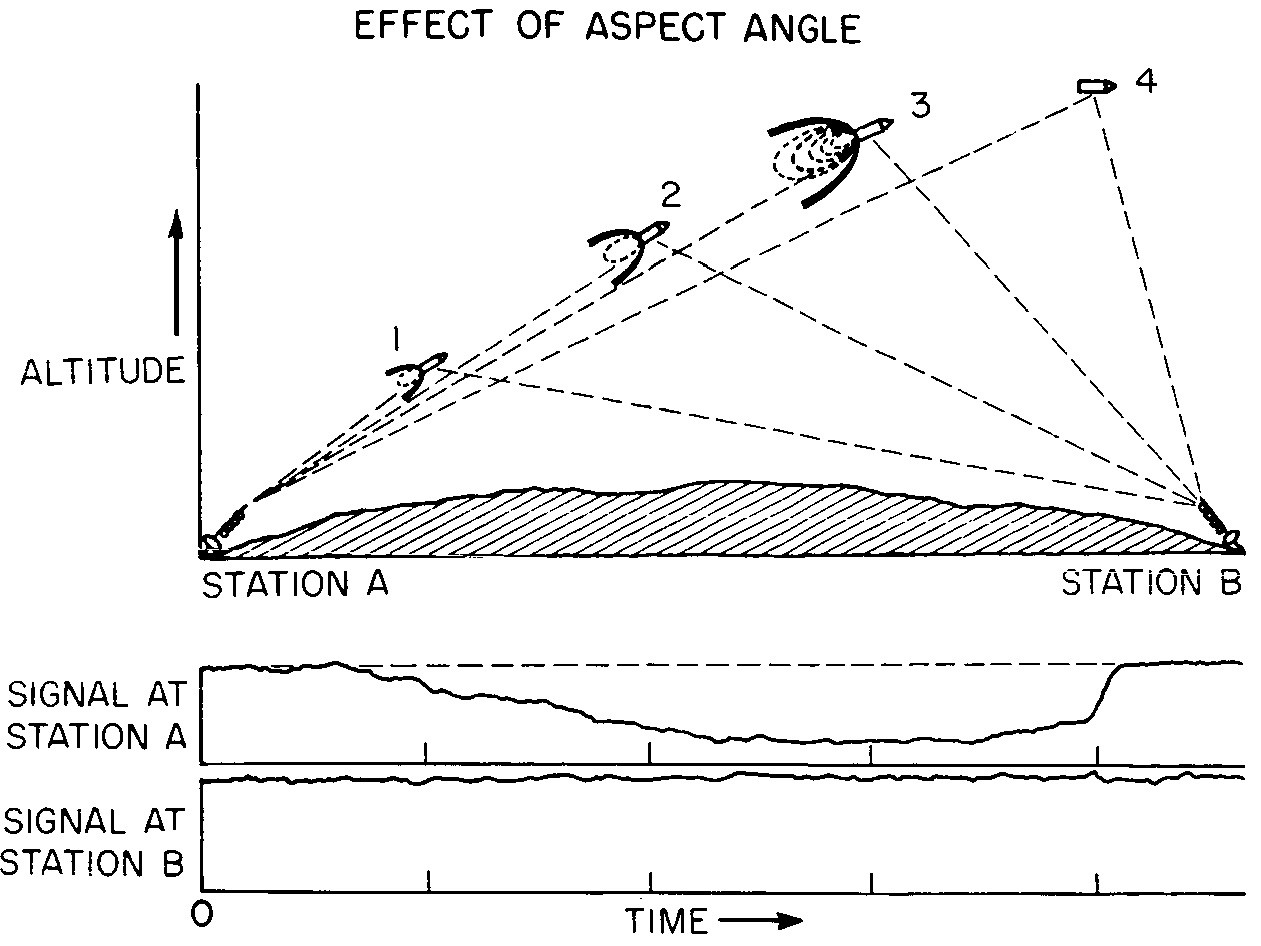
Figure 3: The interplay of flame attenuation, altitude and aspect angle. Illustration taken from page 175 of the declassified NASA paper ‘Proceedings of the NASA Conference on Communicating Trough Plasmas of Atmospheric Entry and Rocket Exhaust’, Langley 1964.

Flame attenuation: If hot enough, a fire will produce plasma through ionization of the gases in its flame. In practice, this leads to a highly variable attenuation when the signal passes through fire, be it from the exhaust of a rocket engine or a bush fire in Australia. This effect is most pronounced when a vehicle travels fast enough to develop a plasma envelope—say, during re-entry—and has been researched by NASA since the 50s (see figure 3).

Rain fade: Frequency dependent scattering due to rain and precipitation in general. Might be modeled as a frequency dependent attenuation.

Pointing loss: Loss due to imperfect antenna aim.

Multipath propagation: Interference effects due to the signal reaching the antenna by several paths of differing lengths. Leads to comb-filtering, i.e. frequency dependent drops and boosts in signal strength.

Polarization mismatch: Loss due to differences in polarization. Might be severe if the receiver and transmitter use orthogonal polarization states.

A note on units

Link analysis calculations are often done in decibel, as the involved quantities typically differ by several orders of magnitude. Decibel is a relative unit of measurement, and physical quantities—like, say, transmitted power $P_\text{TX}$ —must therefore be written as ratios of some fixed reference value before they can be expressed in decibel. It is customary to add a suffix to the decibel symbol indicating the reference value. For power measurements, two references are in common usage: 1 watt, indicated by a suffix ‘W’, and 1 milliwatt, indicated by a suffix ‘m’. Hence, a value of e.g. ’20 dBm’ is a power of about 100 mW. In a similar manner, antenna gain is sometimes given in ‘dBi’, to emphasize that the quoted decibel value is relative to a (lossless) isotropic antenna.

Generally, quantities can be converted back and forth from decibel by

$\displaystyle x_\text{dB} = 10 \log_{10} \! \left( \frac{x}{x_\text{ref}} \right)$

$\displaystyle x = x_\text{ref} \cdot 10^{x_\text{dB}/10} ,$

where $x_\text{ref}$ is the chosen reference value, measured in the same units as $x$ . Using this, we can easily convert the transmission equation given above into decibels:

$\displaystyle P_\text{RX} = P_\text{TX} + G_\text{TX} + G_\text{RX} - L_\text{TX} - L_\text{RX} - L_0 - \sum L ,$

where the free-space path loss in decibels is given by

$\displaystyle L_0 = 20 \log (4 \pi d / \lambda) = 20 \log (4 \pi d f / c).$

<< Previous page – Content – Next page >>

This article is part of a pre-course program used by Andøya Space Education in Fly a Rocket! and similar programs.