Atmospheric Physics

The International Standard Atmosphere

The International Standard Atmosphere is an atmospheric model or convention which is used as a reference when actual atmospheric conditions are to be described.

Variables used for such a description are e.g. pressure, temperature, and the number density of the air molecules. Most significantly, the convention divides the atmosphere into different layers based on the temperature gradient (see figure 1). The table below shows this layering in more detail:

Level	Layer	Altitude [km]	Lapse rate [^oC/km]	Base temperature [^oC]	Static base pressure [Pa]
0	Troposphere	0	−6.5	+15.0	101325
1	Tropopause	11.019	0.0	−56.5	22632
2	Stratosphere	20.063	+1.0	−56.5	5474.9
3	Stratosphere	32.162	+2.8	−4.5	868.02
4	Stratopause	47.350	0.0	−2.5	110.91
5	Mesosphere	51.413	−2.8	−2.5	66.939
6	Mesosphere	71.802	−2.0	−58.5	3.9564
7	Mesopause	86.000	–	−86.2	0.3734

There are more than one ‘reference atmosphere’. The International Standard Atmosphere above is originally the US Standard Atmosphere from 1976 which includes all layers up to the mesopause but neglects the thermosphere.

Stability in a gas

Stability as a concept in physics is easy to understand: A body that is displaced from one (or maybe several) equilibrium position(s) either moves away further (instability), moves back (stability), or does not move at all if another equilibrium position is found.

A gas is no body in the sense the term is used above. It is, however, possible to define the term ‘body’ as a volume of gas, a so-called ‘parcel of air’. This is akin to (but of course not exactly the same) as defining light pulses to be made of particles (photons) in order to be able to calculate certain things about electromagnetic radiation more easily.

Assume that such a parcel of air is located in the troposphere. In equilibrium, it has a certain pressure $p_\text{eq}$ and temperature $T_\text{eq}$ . Assume further that the parcel is pushed upwards until it has pressure $p_1$ and temperature $T_1$ . Based upon what we know about the troposphere we would expect that $p_1 < p_\text{eq}$ and $T_1 < T_\text{eq}$ since both pressure and temperature are supposed to decrease with increasing altitude. In a stable atmosphere, this means that the parcel of air cools such that it eventually will sink again until it has $p_\text{eq}$ and $T_\text{eq}$ .

But what if $p_1 > p_\text{eq}$ , or $T_1 > T_\text{eq}$ , i.e. what if the parcel gains energy from its surroundings while it ascends? This may happen e.g. when a gravity wave propagates through the parcel. Then the parcel of air will be lifted even higher and moves away from its equilibrium position. The movement of the parcel may become unstable. In such a case one uses the term locally unstable atmosphere.

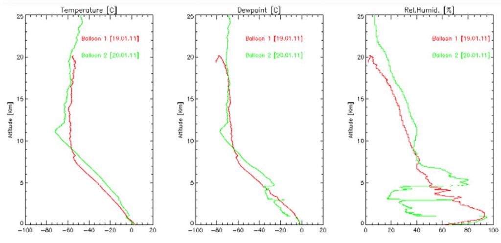
The next figure shows balloon data examples. In the plot to the left, the temperature graph for the balloon 2 shows an increase in temperature at around 1 km height. This cannot be turbulence since we observe a cloud layer at the same height in the plot to the right. Low-altitude clouds/humidity layers cannot exist in an unstable atmosphere. Thus, the temperature increase shows the top of the planetary boundary layer.

Example weather balloon data from Andøya Space.

How to recognize a local instability in the atmosphere

A different way of looking at atmospheric stability is to say that a stable atmosphere resists vertical air motion while an unstable atmosphere does not. Here is the idea:

We define the dry adiabatic lapse rate as the temperature gradient a dry parcel of air would experience while rising and cooling adiabatically. The wet adiabatic lapse rate is then the analogue for a parcel of air which is saturated with water vapour.

Stability arises from energy transfer to the parcel of air, i.e. temperature evolution as the parcel rises is no longer adiabatic. Thus, we can define for any parcel of air that the atmosphere is (1) absolutely stable when the actual temperature gradient or environmental lapse rate is lower than the wet adiabatic lapse rate, (2) absolutely unstable if the temperature gradient is larger than the dry adiabatic lapse rate and (3) conditionally stable if the temperature gradient is larger than the wet but smaller than the dry adiabatic lapse rate.

Planetary Boundary Layer

Atmospheric stability is of major importance in the so-called Planetary Boundary Layer (PBL) which is the atmospheric layer closest to the ground. Here, both friction between air motion and the Earth’s surface, as well as infrared radiation from the Earth’s surface, have such a great degree of influence on the energy balance in the atmosphere that turbulent motion can occur quite often.

The following figure shows the Planetary Boundary Layer within the troposphere. Note, how ‘topography’—i.e. a mountain—can produce turbulence on the lee side.

As is the case with the tropopause (and for mostly the same reason), the thickness of the PBL is variable with latitude. For even if frictional forces due to ‘topography’ are dependent on local conditions and therefore can be assumed to be constant, the amount of energy absorbed and converted into thermal radiation is not. At the equator a lot more of the Sun’s radiation reaches the Earth’s surface, such that the PBL and the troposphere are much thicker than at the poles.

<< Previous page – Content – Next chapter >>

This article is part of a pre-course program used by Andøya Space Education in Fly a Rocket! and similar programs.