Introduction of the six basic parameters describing satellite orbits

A satellite orbit is always in a plane around the heaviest body. The plane contains this body’s center. In this article, we will discuss the six classical orbital elements.

The Orbital Elements

This system has six degrees of freedom. We need six parameters to describe the orbit. Three of the parameters we will use, describe how the plane looks like and the position of the satellite on the ellipse, and the other three parameters will describe how that plane is oriented in the celestial inertial reference frame and where the satellite is in that plane. These six parameters are called the Keplerian elements or orbital elements.

Figure 1: Definition of the semi-major axis a; the semi-minor axis b; the true anomaly θ; and apoapsis and periapsis, with their respecitve radii r_a and r_p. Illustration by Andøya Space Education.

Semi-Major and Semi-Minor Axis

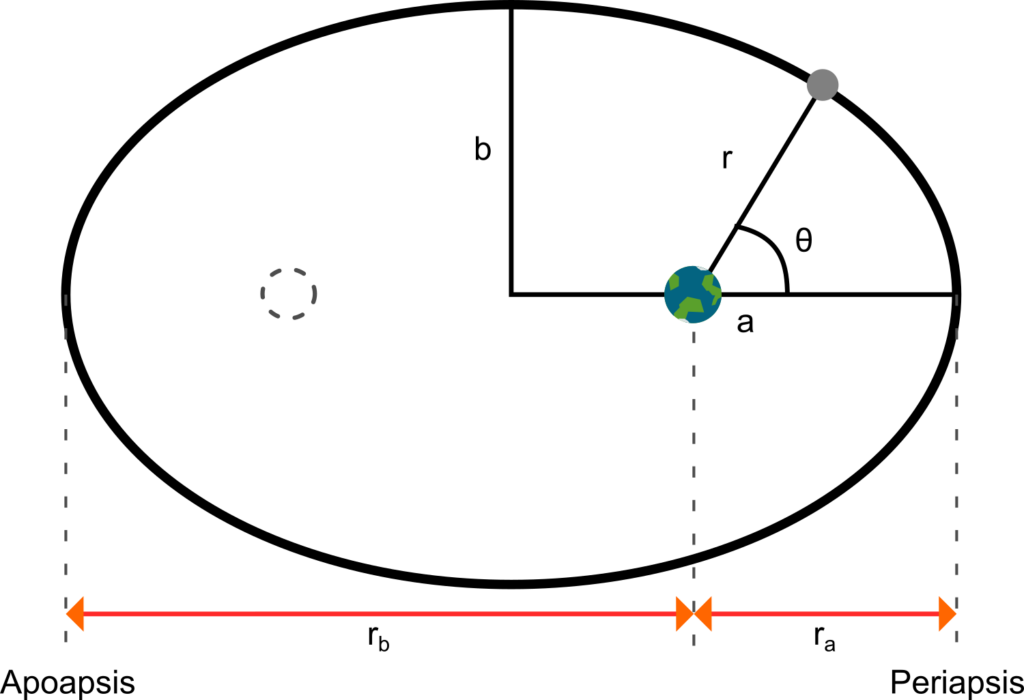
The general elliptical orbit of a satellite orbiting a planet is seen in figure 1. The heaviest body in the Keplerian orbit (here, a planet), is in one of the focal points of the ellipse of the orbiting satellite (grey disk). The other focal point is empty and is here marked with a dashed circle. The shortest radius in the ellipse is the semi-minor axis $b$ and the largest radius is the semi-major axis $a$ . Both distances are measured from the center of the ellipse. The semi-major axis $a$ is the first Keplerian parameter, which we will use to describe the size of the ellipse.

In the case of man-made satellites, it is often practical to relate the parameters to what we measure from Earth, and not some arbitrary empty point in space. Generally, the point where the satellite is the closest to the central body is called the periapsis, with the length to the central body usually denoted as $r_\text{p}$ . The point where the satellite is the farthest away is called the apoapsis, and has the associated length $r_\text{a}$ . The semi-major axis is on the line segment between the periapsis and the apoapsis, and it is half of the distance between them, that is $a = (r_\text{p} + r_\text{a})/2$ .

Eccentricity

We have now given a parameter of the size of the orbit, but to completely define the orbit we also need to know it’s shape. This is given by the second orbital parameter, the eccentricity $e$ . It can be defined from $r_\text{p}$ and $r_\text{a}$ , and is quite simple to calculate. For an elliptical orbit it is given as

$e = \dfrac{r_\text{a} - r_\text{p}}{r_\text{a} + r_\text{p}}.$

It does not matter what units the two radii are given in as the eccentricity is unitless. As an example, what is the eccentricity of a circle? Since a circle has constant radius, we must have that $r_\text{a} = r_\text{p}$ making the eccentricity $e=0$ . An ellipse will have an eccentricity from $e = 0$ up to (but not including) $e=1$ . What kind of orbits we get for even higher eccentricities, we will come back to shortly. Ellipses with different eccentricities are shown in figure 2.

Figure 2: Eccentricities in orbits where one of the focal points is fixed, as well as the periapsis radius. Eccentricities from 0 to 0.9 are shown to increase in steps of 0.1. Note that neither the semi-major axis a nor the semi-minor axis b is constant here. Illustration by Andøya Space Education.

In figure 1 we can see that the radius r is given from the central body to the center of the satellite. The angle $\theta$ is the angle between the semi-major axis and the line between the central body to the satellite and varies in time when the satellite orbits the central body. When the satellite is at perigee the angle is $0^\circ$ and when it is at apogee the angle is $\theta = 180^\circ$ . The angle $\theta$ is most often called the true anomaly and is the third orbital parameter. It describes the orbital position of the satellite at any specific time.

Now we have found the first three parameters describing the orbit and the satellite position in it. The following expression

$r = \dfrac{a(1-e^2)}{1+e\cos \theta}$

describes the orbit in polar coordinates as a function of the true anomaly. We stated previously that ellipses have eccentricities from 0 up to 1, and for these cases the radius will be well defined for all angles $\theta$ as can easily be seen.

Figure 3: Definition of the true and eccentric anomalies ( $\theta$ and $E$ , respectively). Illustration derived from a derived work by the Wikimedia-user CheChe (original by Brews ohare). Licenced under CC BY-SA 4.0.

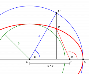
The true anomaly is one of the three anomalies/parameters describing the position around the orbit. The other two anomalies are called the eccentric anomaly and mean anomaly, and they are used to relate the position of the satellite (from the true anomaly) to the time since the passing of the perigee. The eccentric anomaly $E$ is an actual angle shown in figure 3. The position of the satellite is at the point P with true anomaly $\theta$ . The blue (largest) circular orbit has a constant radius equal to the semi-major axis $a$ of the satellite orbit (shown in red in the figure). The eccentric anomaly is the left angle $E$ in the triangle CQP’, where the line segment QP’ is the line segment perpendicular to the periapsis–apoapsis line through the point P (the actual position of the satellite) to the point P’, which is the intersection with the circular blue orbit (the point Q is not marked on the figure). This makes the length of the hypotenuse (the line segment CP’) the satellite semi-major axis. The relation between the true anomaly $\theta$ and the eccentric anomaly is

$\tan \! \left( \dfrac{\theta}{2} \right) = \sqrt{\dfrac{1+e}{1-e}} \; \tan \! \left( \dfrac{E}{2} \right) .$

The mean anomaly $M$ is not a true angle. It is defined as $M= t_\text{p} \, n$ where $t_\text{p}$ is the time since the last crossing of periapsis and $n = 2\pi/T = 360^\circ /T$ , where $T$ is the orbital period of the satellite orbit. The mean anomaly is an angle an imaginary satellite would have if it where in a circular orbit around the point C (figure 3) with a time period $T$ equal to the true satellite orbit. The reason of why we define the eccentric and mean anomaly is to find the relationship between the true anomaly and the time since periapsis. The relationship between the mean and eccentric anomaly is

$M = E - e \sin (E),$

where $e$ is the eccentricity of the (true) satellite orbit. This equation is a transcendental equation that cannot be solved analytically for $E,$ but several resources online can help with solving equations like this, e.g. WolframAlpha.com. Knowing the true anomaly, the time since periapsis can be found by first calculating the eccentric anomaly and then the mean anomaly. Knowing the time since periapsis, however, the mean anomaly is first calculated, but finding the eccentric anomaly need to be found numerically. That solution is then used to find the true anomaly.

Non-eliptic orbits

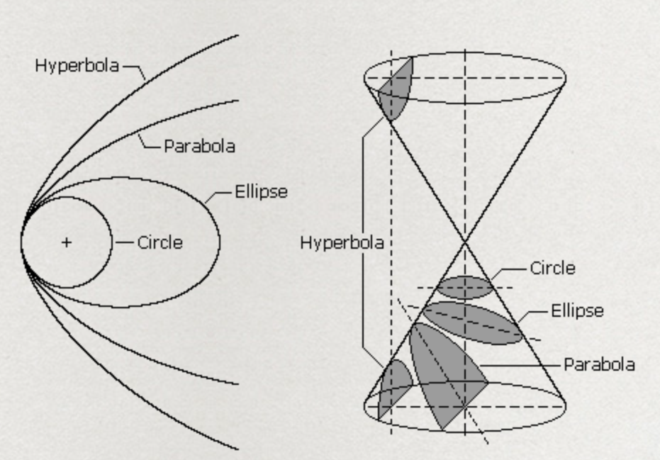
Orbit in space — Figure 4: Orbits as conic sections. Credits: Robert A. Braeunig.

Orbits with $e=1$ are called parabolas, while orbits with higher eccentricity (i.e. $e > 1$ ) are called hyperbolas. These orbits have an infinitely long orbital period—they never return to a point they have already been at, because they have a higher velocity than the escape velocity (parabolas actually have exactly the escape velocity). Some comets observed from Earth travel along such orbits, but satellites very seldomly do. These are thus special cases, which we will not discuss further.

Parameters used to describe the orientation in space

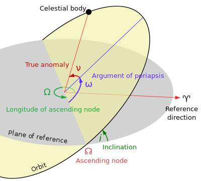
orbital-elements — Figure 5: The orbital elements. Source: Wikimedia.

We use the celestial reference frame to define some additional parameters. See figure 5. The angle between the elliptical plane and the reference plane is called the inclination $i$ , and is measured from the reference plane to the orbital plane at the ascending node. The inclination is the first orbital parameter which describes the orientation of the orbit. The second parameter $\omega$ is the argument of periapsis, also called the argument of perigee, and is the angle between the ascending node and the semi-major axis of the ellipse. The last orbital parameter is the longitude of ascending node $\Omega$ , which is the angle between the reference direction and the ascending node in the travelling direction of the satellite from the ascending node (counter-clockwise as seen in the figure).

The six orbital parameters are shown in the video below:

A closer description of the orbital parameters is given in this video, but note that a different base angle is used in the true anomaly:

Finding orbital parameters from observation

It is impractical to have to wait until the satellite reaches its apogee and perigee to measure it, and we instead want a method where we can find the orbital parameters from observations at different, arbitrary orbital positions.

There are numerous ways of doing this. We will follow the so-called Gibbs method. This method takes three different positions along the orbit, and for one of those positions it calculates the velocity. From three-dimensional position and velocity vectors at a given time one can calculate all the orbital parameters discussed above. The method will here be given as an algorithm without explaining the background. The method is described well in the literature. Curtis’ Orbital Mechanics for Engineering Students (2010), for example, gives an excellent introduction to this and other techniques.

We have three position vectors $\vec{r}_1,$ $\vec{r}_2$ and $\vec{r}_3$ along the orbit.

Find the absolute value of the three vectors (i.e. the distance from the focal point to the satellite), $r = || \vec{r} || = \sqrt{r_x^2 + r_y^2 + r_z^2}$ .
Calculate $\vec{N} = r_1 \left( \vec{r}_2 \times \vec{r}_3 \right) + r_2 \left( \vec{r}_3 \times \vec{r}_1 \right) + r_3 \left( \vec{r}_1 \times \vec{r}_2 \right)$ , where $\times$ is the cross product.
Calculate $\vec{D} = \vec{r}_1 \times \vec{r}_2 + \vec{r_2} \times \vec{r}_3 + \vec{r}_3 \times \vec{r}_1$ .
Calculate $\vec{S} = \vec{r}_1 \left( r_2 - r_3 \right) + \vec{r}_2 \left( r_3 - r_1 \right) + \vec{r}_3 \left( r_1 - r_2 \right)$ .
The velocity in the position $\vec{r}_2$ is then $\vec{v}_2 = \sqrt{\dfrac{\mu}{N D}} \left( \dfrac{\vec{D} \times \vec{r}_2}{r_2} + \vec{S} \right)$ , where $\mu = G M$ is called the gravitational parameter. For Earth, $\mu_\text{E} \approx 398.6 \times 10^{12} \,\text{ m}^3/\text{s}^2 = 398 \, 600 \,\text{km}^3/\text{s}^2$ .

Note that there is a difference between a vector (with an arrow) and the length of the vector. The vectors $\vec{r}$ and $\vec{v}$ combined are called the state vector. From this, we can calculate all the different parameters expanding on that algorithm:

First find the tangential velocity component by $v_r = \dfrac{\vec{r} \cdot \vec{v}}{r}$ .
Then find the eccentricity vector $\vec{e} = \left( \dfrac{v^2}{\mu} - \dfrac{1}{r} \right) \vec{r} - \dfrac{r v_r}{\mu} \vec{v}$ . The length of $\vec{e}$ is the well-known eccentricity $e$ .
The true anomaly $\theta$ at $\vec{r}_2$ is given by $\cos ( \theta ) = \dfrac{\vec{e}}{e} \cdot \dfrac{\vec{r}}{r}$ , assuming the radial velocity is positive (including 0). If the radial velocity is less than zero, replace $\cos (\theta)$ with $\cos \left(360^\circ - \theta \right)$ .
From the equation of motional energy (introduced later in this chapter), we find the semi-major axis by $a = -\dfrac{\mu}{v^2 - 2\frac{\mu}{r}}$ .
For reference we also find the three parameters describing the plane orientation. First find the specific angular momentum $\vec{h} = \vec{r} \times \vec{v}$ . Then find the vector $\vec{N} = \hat{k} \times \vec{r}$ where $\hat{k} = ( 0, \, 0, \, 1 )$ is the unit vector in z direction.
The inclination $i$ is calculated from $\cos (i) = h_Z/h$ .
The right ascension of the ascending node (RAAN) / longitude of the ascending node, $\Omega$ , is calculated from $\cos ( \Omega ) = \cos \left( \dfrac{N_X}{N} \right)$ , provided that $N_y \geq 0$ . If $N_y < 0$ , replace $\cos (\Omega)$ with $\cos \left(360^\circ - \Omega \right)$ . For non-inclined orbits (where $i=0^\circ$ ), the RAAN is conventionally set to $0^\circ$ .
For non-zero inclinations, the argument of perigee is calculated from $\cos \left( \omega \right) = \dfrac{\vec{N}}{N} \cdot \dfrac{\vec{e}}{e}$ . When the inclination is zero, the argument of perigee is found using $\tan ( \omega ) = \dfrac{e_y}{e_x}$ , since $\vec{N} \cdot \vec{e} = 0$ when $i = 0^\circ$ .

<< Previous page – Content – Next page >>

This article is part of a pre-course program used by Andøya Space Education in Fly a Rocket! and similar programs.