Three types of orbits are of particular interest: low Earth orbits (LEO), which goes up to about 2000 km; medium Earth orbits (MEO), which are between LEO and GEO (see below); and geostationary Earth orbits (GEO), which are at 42 164 km. Hardly any satellites orbit Earth above GEO (with one notable exception, which will be discussed later).
Most satellites in LEO orbits above 300 km, where the reduced atmospheric drag makes it possible to maintain a reasonably stable altitude without spending too much fuel on orbital maintenance. Nonetheless, periodic burns are needed. The International Space Station (ISS) orbits at 350–400 km, and its altitude is chosen as a trade-off between the cost of reaching orbit and the fuel needed to be transported for altitude maintenance. The ISS has an inclination of about 52 degrees, making it easier to reach from the USA and Russia which frequently send cargo and astronauts. Above 500–600 km the atmospheric drag is negligible, allowing satellites to stay in orbit for years without ever needing to compensate for the drag.
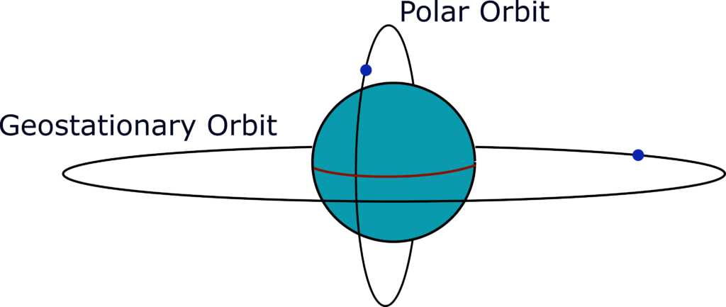
A geostationary satellite orbits Earth once every sidereal day (about 23 hours and 56 minutes, since the Earth moves around the Sun while rotating around its own axis). This means that the satellite, as viewed from Earth, stays still above a fixed location on the ground. This make it much easier to receive TV signals and communication from it, as practically no tracking is needed.
Another important orbit is at about 20 000 km of altitude (orbital period of approx. 12 hours), where most global navigation satellite system constellations are found.
The last satellite orbit we will discuss is not an orbit that satellites operate in, but merely a way of transportation to its final orbit. This orbit is called a Hohmann orbit, see figure 2. Imagine a satellite launched into a circular orbit of 350 km altitude. The satellite is intended to reach a circular orbit with an altitude of 5000 km. The satellite at 350 km altitude increases its orbit with a change in velocity of  and this changes the orbit to an elliptical orbit with perigee at 350 km and apogee at 5000 km since
  is carefully calculated in advance. After half an orbital period the satellite reaches the apogee, where it does a second burn with
  to change the orbit once again to a circular orbit. See figure 2.
Note that Hohmann orbits can be used both to increase and decrease orbital altitude, but that the initial and final orbits need to be both circular and co-planar (and also co-focal, i.e. orbiting the same point). Although this definition seemingly makes Hohmann transfers entirely academic (since no real orbits are ever perfectly circular and co-planar), it turns out that the same idea also works well—with some modifications—for elliptical initial and final orbits. The main difference to keep in mind is that maximum efficiency is obtained if the initial and final orbits are oriented such that the first burn raises the old apoapsis to the new apoapsis and the second burn the old periapsis to the new periapsis (or in reverse order, if decending). As long as the ratio between the lower and higher semi-major axis is not too large, such a ‘generealized Hohmann transfer’ is the most efficient simple transfer orbit.
In practice, satellites intended for orbits higher than low LEO are usually launched straight into a Hohmann orbit. One example is the geostationary transfer orbits (GTO), which carry communication satellites to GEO. Launching straight into GTO means that the satellite only needs to burn its motors once, upon reaching the desired GEO apogee (this technique is known as ‘orbital insertion’).
See how astronauts reach the ISS in this video:
GTO has a semi-major axis of  Using the energy conservation formula
  , we can write

For an apogee at  , we find the velocity

The orbital velocity at GEO (at the same altitude) is

The change in velocity, , needed for orbital injection to GEO is therefore

For a satellite with an initial wet mass (including fuel) of 4 000 kg and a motor with  , the final fuel after burn is

making the propellant needed for the insertion 
After orbital injection, the satellite needs some propellants for station keeping, burning the motors to compensate for secondary effects. Some of these effects is accounting for Earth not being perfectly spherical, sun pressure and gravitational forces from other celestial objects. After the end of life of a geostationary satellite, being that GEO is such an important object for the modern society, the satellites is moved to a higher orbit called a graveyard orbits only used for decommissioned satellites.
<< Previous page – Content – Next chapter >>
This article is part of a pre-course program used by Andøya Space Education in Fly a Rocket! and similar programs.